Exercise set 9: Double machine learning

In this exercise set we will once again be working with estimation of conditional average treatment effects assuming selection on observables. However, this time the focus will be more broadly on double machine learning in econml, learning how to utilize these methods to get estimates, both assuming a partially linear model (LinearDML) and non-parametrically using causal forests (CausalForestDML).

As an example we will examine the age-old question of orange juice price-elasticity, which, as we all know, have haunted economists for millenia. To answer this question we will use a subset of Dominick’s dataset from the James M. Kilts Center, University of Chicago Booth School of Business. The data is a repeated cross sectional from stores (which we pool), where our main variables of interest are the amount of units sold (outcome) and the price of orange juice (treatment) and median income in the neighborhood (treatment effect heterogeneity). A description of the dataset can be seen here. Throughout, we assume selection on observables. This exercise was in part inspired by the econml notebooks on causal model selection and double machine learning.

import matplotlib.pyplot as plt
import numpy as np 
import pandas as pd 
import os
import urllib.request

## Ignore warnings
import warnings
warnings.filterwarnings("ignore")

# Set seed and plot style
np.random.seed(73)
plt.style.use('seaborn-whitegrid')

%matplotlib inline

Getting started

In this first part of the exercise we will be digging straight into estimating treatment effects using double machine learning. As such, we will be postponing training of models for predicting Y and T for just a moment, although this is an essential part of double machine learning and should not be neglected.

Exercise 1.1

Load the data using the following code and verify that you have correctly loaded the DataFrame by printing the first 5 rows.

NOTE: The following code will download the file which might take a few seconds dependent on your internet.

Hints:

DataFrame’s have a method called .head()

# Import the data
file_name = "oj_large.csv"

if not os.path.isfile(file_name):
    print("Download file")
    urllib.request.urlretrieve("https://msalicedatapublic.blob.core.windows.net/datasets/OrangeJuice/oj_large.csv", file_name)
    
oj_data = pd.read_csv(file_name)

### BEGIN SOLUTION

oj_data.head()

### END SOLUTION

	store	brand	week	logmove	feat	price	AGE60	EDUC	ETHNIC	INCOME	HHLARGE	WORKWOM	HVAL150	SSTRDIST	SSTRVOL	CPDIST5	CPWVOL5
0	2	tropicana	40	9.018695	0	3.87	0.232865	0.248935	0.11428	10.553205	0.103953	0.303585	0.463887	2.110122	1.142857	1.92728	0.376927
1	2	tropicana	46	8.723231	0	3.87	0.232865	0.248935	0.11428	10.553205	0.103953	0.303585	0.463887	2.110122	1.142857	1.92728	0.376927
2	2	tropicana	47	8.253228	0	3.87	0.232865	0.248935	0.11428	10.553205	0.103953	0.303585	0.463887	2.110122	1.142857	1.92728	0.376927
3	2	tropicana	48	8.987197	0	3.87	0.232865	0.248935	0.11428	10.553205	0.103953	0.303585	0.463887	2.110122	1.142857	1.92728	0.376927
4	2	tropicana	50	9.093357	0	3.87	0.232865	0.248935	0.11428	10.553205	0.103953	0.303585	0.463887	2.110122	1.142857	1.92728	0.376927

Exercise 1.2

The following code subsets the data into different parts corresponding to X, Y, W and T, but have been named temporary names. Which is which, and why?

Hints:

What’s just confounders and what drives heterogeneity?

# Prepare data

from sklearn.preprocessing import StandardScaler
from sklearn.model_selection import train_test_split

scaler = StandardScaler()

non_categorical_cols = ['feat', 'AGE60', 'EDUC', 'ETHNIC', 'HHLARGE', 'WORKWOM', 'HVAL150', 'SSTRDIST', 'SSTRVOL', 'CPDIST5', 'CPWVOL5']
categorical_cols = ['brand']

temp_1 = scaler.fit_transform(oj_data[non_categorical_cols].values)
temp_2 = scaler.fit_transform(pd.get_dummies(oj_data[categorical_cols]).values)
# Stacks categorical and non categorical variables together
temp_3 = np.hstack([temp_1, temp_2]) 
temp_4 = np.log(oj_data["price"]).values
temp_5 = oj_data['logmove'].values
temp_6 = scaler.fit_transform(oj_data[['INCOME']].values)

X = # FILL IN
W = # FILL IN
Y = # FILL IN
T = # FILL IN

XW = np.hstack([X, W])

Y_train, Y_val, T_train, T_val, X_train, X_val, W_train, W_val, XW_train, XW_val = train_test_split(Y, T, X, W, XW, test_size=.2)

# Prepare data

from sklearn.preprocessing import StandardScaler
from sklearn.model_selection import train_test_split

scaler = StandardScaler()

non_categorical_cols = ['feat', 'AGE60', 'EDUC', 'ETHNIC', 'HHLARGE', 'WORKWOM', 'HVAL150', 'SSTRDIST', 'SSTRVOL', 'CPDIST5', 'CPWVOL5']
categorical_cols = ['brand']

temp_1 = scaler.fit_transform(oj_data[non_categorical_cols].values)
temp_2 = scaler.fit_transform(pd.get_dummies(oj_data[categorical_cols]).values)
temp_3 = np.hstack([temp_1, temp_2])

temp_4 = oj_data['logmove'].values
temp_5 = np.log(oj_data["price"]).values

temp_6 = scaler.fit_transform(oj_data[['INCOME']].values)

X = temp_6
W = temp_3
Y = temp_4
T = temp_5

XW = np.hstack([X, W])

Y_train, Y_val, T_train, T_val, X_train, X_val, W_train, W_val, XW_train, XW_val = train_test_split(Y, T, X, W, XW, test_size=.2)

Exercise 1.3

Create an instance of a LinearDML and fit it to the training data using default input parameters.

Hints:

There’s an example on this page

# Your code

### BEGIN SOLUTION

from econml.dml import LinearDML

linear_est = LinearDML()
linear_est.fit(Y_train, T_train, X=X_train, W=W_train)

### END SOLUTION

<econml.dml.dml.LinearDML at 0x2a1b2632f50>

Exercise 1.4

Look at the documentation for LinearDML, which can be found here.

How are the models for Y and T created? Does this explain why the data was scaled?

# Your answer

### BEGIN SOLUTION

# cross validated LASSO -- sensitive to scaling, hence standardscaling!

### END SOLUTION

Exercise 1.5

Get an estimate of the treatment effect heterogeneity using the summary method. Is the sign as expected?

# Your code

### BEGIN SOLUTION

linear_est.summary()

# Positive slope -- less price sensitive as income increases. Makes sense!

### END SOLUTION

Coefficient Results

	point_estimate	stderr	zstat	pvalue	ci_lower	ci_upper
X0	0.155	0.027	5.821	0.0	0.102	0.207

CATE Intercept Results

	point_estimate	stderr	zstat	pvalue	ci_lower	ci_upper
cate_intercept	-2.601	0.026	-98.624	0.0	-2.652	-2.549

_{A linear parametric conditional average treatment effect (CATE) model was fitted:
$Y = \Theta(X)\cdot T + g(X, W) + \epsilon$
where for every outcome $i$ and treatment $j$ the CATE $\Theta_{ij}(X)$ has the form:
$\Theta_{ij}(X) = X' coef_{ij} + cate\_intercept_{ij}$
Coefficient Results table portrays the $coef_{ij}$ parameter vector for each outcome $i$ and treatment $j$. Intercept Results table portrays the $cate\_intercept_{ij}$ parameter.}

Exercise 1.6

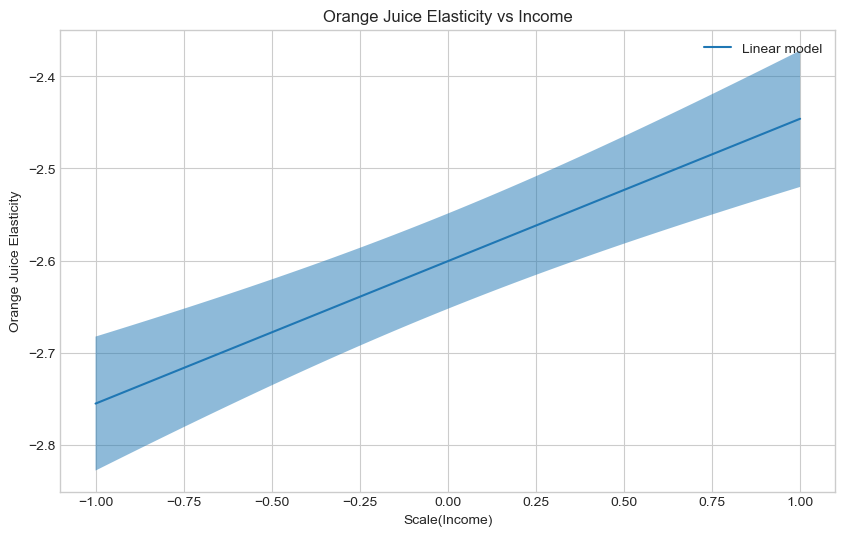
Estimate and plot the conditional average treatment effect and the the 95% confidence interval with the LinearDML model on the following X_test data, which generates counterfactual income levels ranging from -1 to 1.

Hints:

There documentation for LinearDML can be found on this page.

Try looking for methods that start with effect

## Generate test data
min_income = -1
max_income = 1
delta = (1 - (-1)) / 100
X_test = np.arange(min_income, max_income + delta - 0.001, delta).reshape(-1,1)

# Calculate treatment effect and interval

te_pred_linear = # FILL IN 
te_pred_interval_linear = # FILL IN 

# Plot Orange Juice elasticity as a function of income

plt.figure(figsize=(10,6))
plt.plot(X_test, te_pred_linear, label="Linear model")
plt.xlabel(r'Scale(Income)')
plt.ylabel('Orange Juice Elasticity')
plt.legend()
plt.title("Orange Juice Elasticity vs Income")
plt.show()

SyntaxError: invalid syntax (1647766146.py, line 9)

### BEGIN SOLUTION

# Generate test data
min_income = -1
max_income = 1
delta = (1 - (-1)) / 100
X_test = np.arange(min_income, max_income + delta - 0.001, delta).reshape(-1,1)

# Calculate treatment effects

te_pred_linear = linear_est.effect(X_test)
te_pred_interval_linear = linear_est.effect_interval(X_test, alpha = 0.05)

# Plot Orange Juice elasticity as a function of income

plt.figure(figsize=(10,6))
plt.plot(X_test, te_pred_linear, label="Linear model")
plt.fill_between(X_test.flatten(), te_pred_interval_linear[0], te_pred_interval_linear[1], alpha=.5)
plt.xlabel(r'Scale(Income)')
plt.ylabel('Orange Juice Elasticity')
plt.legend()
plt.title("Orange Juice Elasticity vs Income")
plt.show()

### END SOLUTION

Exercise 1.7

Create an instance of a CausalForestDML and fit it to the training data using default input parameters.

Hints:

It follows exactly the same recipe as LinearDML.

# Your code

### BEGIN SOLUTION

from econml.dml import CausalForestDML

cf_est = CausalForestDML()
cf_est.fit(Y_train, T_train, X=X_train, W=W_train)

### END SOLUTION

<econml.dml.causal_forest.CausalForestDML at 0x2a1b97de3e0>

Exercise 1.8

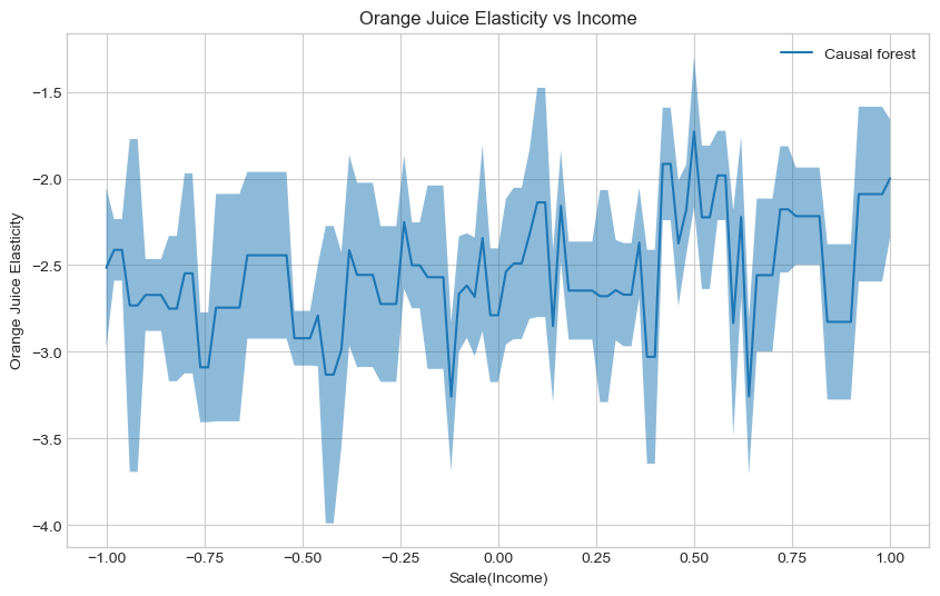
Estimate and plot the conditional average treatment effect and the the 95% confidence interval with the CausalForestDML model X_test.

Hints:

It follows exactly the same recipe as LinearDML.

# Your code

### BEGIN SOLUTION

te_pred_cf = cf_est.effect(X_test)
te_pred_interval_cf = cf_est.effect_interval(X_test, alpha=0.05)

# Plot Orange Juice elasticity as a function of income
plt.figure(figsize=(10,6))


plt.plot(X_test, te_pred_cf, label="Causal forest")
plt.fill_between(X_test.flatten(), te_pred_interval_cf[0], te_pred_interval_cf[1], alpha=.5)
plt.xlabel(r'Scale(Income)')
plt.ylabel('Orange Juice Elasticity')
plt.legend()
plt.title("Orange Juice Elasticity vs Income")
plt.show()

### END SOLUTION

As discussed during the lecture, we can use the R-loss to evaluate the fit of the conditional average treatment effect and use this to perform causal model selection.

This could be done manually, but much like grf in R, econml also offers automatic tuning with the tune method, which we will utilize to tune the causal forest in CausalForestDML.

Exercise 1.9

Create an instance of a CausalForestDML, tune it on the training data and then fit it to the training data, all using default input parameters.

Hints:

The call to tune the model looks exactly like the call to fit the model.

# Your code

### BEGIN SOLUTION

from econml.dml import CausalForestDML

cf_tuned_est = CausalForestDML()
cf_tuned_est.tune(Y_train, T_train, X=X_train, W=W_train)
cf_tuned_est.fit(Y_train, T_train, X=X_train, W=W_train)

### END SOLUTION

<econml.dml.causal_forest.CausalForestDML at 0x2a1b9beb280>

Exercise 1.8

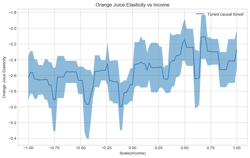
Estimate and plot the conditional average treatment effect and the the 95% confidence interval with the tuned CausalForestDML model on X_test.

Hints:

It follows exactly the same recipe as LinearDML and an untuned CausalForestDML.

# Your code

### BEGIN SOLUTION

te_pred_tuned_cf = cf_tuned_est.effect(X_test)
te_pred_interval_tuned_cf = cf_tuned_est.effect_interval(X_test, alpha=0.05)


# Plot Orange Juice elasticity as a function of income
plt.figure(figsize=(10,6))

plt.plot(X_test, te_pred_tuned_cf, label="Tuned causal forest")
plt.fill_between(X_test.flatten(), te_pred_interval_tuned_cf[0], te_pred_interval_tuned_cf[1], alpha=.5)
plt.xlabel(r'Scale(Income)')
plt.ylabel('Orange Juice Elasticity')
plt.legend()
plt.title("Orange Juice Elasticity vs Income")
plt.show()

### END SOLUTION

Exercise 1.9

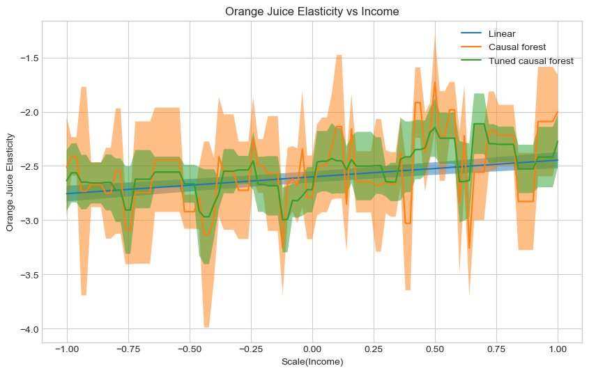
Plot the conditional average treatment effect and the the 95% confidence interval for all three models on X_test. Which do your prefer?

Hints:

You can call plot and fill_between repeatedly before calling xlabel

### BEGIN SOLUTION

# Plot Orange Juice elasticity as a function of income
plt.figure(figsize=(10,6))

# Linear
plt.plot(X_test, te_pred_linear, label="Linear")
plt.fill_between(X_test.flatten(), te_pred_interval_linear[0], te_pred_interval_linear[1], alpha=.5)
# Untuned CF
plt.plot(X_test, te_pred_cf, label="Causal forest")
plt.fill_between(X_test.flatten(), te_pred_interval_cf[0], te_pred_interval_cf[1], alpha=.5)
# Tuned CF
plt.plot(X_test, te_pred_tuned_cf, label="Tuned causal forest")
plt.fill_between(X_test.flatten(), te_pred_interval_tuned_cf[0], te_pred_interval_tuned_cf[1], alpha=.5)
# Make pretty
plt.xlabel(r'Scale(Income)')
plt.ylabel('Orange Juice Elasticity')
plt.legend()
plt.title("Orange Juice Elasticity vs Income")
plt.show()

# No clear way to tell which is the correct model.
# Given that the tuned causal forest is tuned using the R-loss, 
# I would atleast prefer that over the untuned causal forest

### END SOLUTION

Exercise 1.10

econml implements a scoring function using the R-loss, called the Rscorer. Fit the Rscorer to the appropriate data sample.

NOTE: The Rscorer needs a model to create residuals. Here we input a LassoCV, which is also the default in the double machine learning models. As such we obtain similar residuals.

Hints:

Should we use training data or held out data for causal model selection?

# Import model
from sklearn.linear_model import LassoCV
from econml.score import RScorer

# Create scorer
scorer = RScorer(model_y=LassoCV(), model_t=LassoCV())

# FILL IN

### BEGIN SOLUTION

# Import model
from sklearn.linear_model import LassoCV
from econml.score import RScorer

# Create scorer
scorer = RScorer(model_y=LassoCV(), model_t=LassoCV())

scorer.fit(Y_val, T_val, X=X_val, W=W_val)

### END SOLUTION

<econml.score.rscorer.RScorer at 0x2a1b99706d0>

Exercise 1.11

Score the models using the Rscorer’s best_model method. Which model is the preferred one? Is it preferred over a constant average treatment effect?

Hints:

If you’re in doubt as to which model the method has selected, you can return all the scores by setting return_scores = True and compare the best score to the list

The best_model method accepts a list of fitted estimators, and the documentation can be seen here

# Your code

### BEGIN SOLUTION

cate_models = [linear_est, cf_est, cf_tuned_est]
best_model, best_score, score_list = scorer.best_model(cate_models, return_scores = True)

print(best_model)
print(best_score)
print(score_list)

# The tuned causal forest is the best model, 
# As it has an rscore of higher than 0, it is preferred over a constant average treatment effect. 
# Although we note that this is very close to zero

### END SOLUTION

<econml.dml.causal_forest.CausalForestDML object at 0x000002A1B9BEB280>
0.0011816363186031298
[0.0009297028164834131, -0.001814529865579395, 0.0011816363186031298]

Predicting treatment and outcome

Having now looked closer at how to code up estimation of heterogeneous treatment effects using double machine learning estimators, we will start with the task that is predicting both Y and T, from which we can learn the optimal hyperparameters to pass on to our double machine learning estimators.

In practice, this is probably where you will be spending most of the time, optimizing features and models to accurately predict treatment and outcome, thus achieving better converge rates.

We have covered this in both session 3 and 4, where we covered model selection and supervised learning, respectively.

Exercise 2.1

What covariates should we use to predict Y and T? Is this part of the train test split we made in exercise 1.1?

Hints:

Look at the struqtural equations in the lecture slides. What enters in the nuisance functions?

### BEGIN SOLUTION

# Both Y and T should be predicted using both X and W
# If T was used in predicting Y, we should use a doubly robust estimator, which is not possible for continuous outcomes
# We did perform a horizontal stacking of X and W, called XW, before making our train test split
# We can use XW to create the models

### END SOLUTION

To make this go by slightly faster, I have pre-selected three models and their respective hyperparametergrids for which to search over. Furthermore, we utilize 2 fold cross validation (matching the default amount of folds in econml) and 10 random hyperparameter combinations using RandomizedSearchCV, which we covered in session 3.

Each model should be using negative_mean_squared_error, and you should make note of the best performing hyper mean squared error, such that you can compare performance across estimators.

Exercise 2.2

Create a Lasso to predict the outcome, Y.

Save the best hyperparameter combination.

Hints:

The best score and best hyperparameter can be found using the methods best_score_ and best_param_ respectively.

from sklearn.model_selection import RandomizedSearchCV
from sklearn.pipeline import Pipeline
from sklearn # FILL IN 

pipe_lasso = Pipeline([ 
    # FILL IN 
    ]
    )

param_grid = {'lasso__alpha':np.logspace(-5, 3, 10)}


rs = RandomizedSearchCV(
    # FILL IN
)

# Fit
# FILL IN

# Score
# FILL IN

SyntaxError: invalid syntax (3612000372.py, line 5)

### BEGIN SOLUTION

from sklearn.model_selection import RandomizedSearchCV
from sklearn.pipeline import Pipeline
from sklearn.linear_model import Lasso

pipe_lasso = Pipeline([ 
    ('lasso', Lasso(random_state=1))
    ]
    )

param_grid = {'lasso__alpha':np.logspace(-5, 3, 10)}


rs = RandomizedSearchCV(estimator=pipe_lasso, 
                  param_distributions=[param_grid], 
                  scoring='neg_mean_squared_error', 
                  cv=2,
                  n_iter = 10,
                  n_jobs=-1,
                  random_state=73)


# Fit
rs.fit(XW_train, Y_train)

# Score
print(rs.best_params_)
print(rs.best_score_)

y_lasso_best_params = rs.best_params_

### END SOLUTION

{'lasso__alpha': 0.0005994842503189409}
-0.7015673056724774

Exercise 2.3

Create a RandomForestRegressor to predict the outcome, Y.

Save the best hyperparameter combination.

Hints:

The best score and best hyperparameter can be found using the methods best_score_ and best_param_ respectively.

from sklearn # FILL IN

pipe_forest = Pipeline([                     
    # FILL IN
    ]
    )


param_grid= [{
    'forest__n_estimators': np.unique(np.logspace(0, 3, 25).astype(int)),
    'forest__max_features': np.arange(0.1, 1.01, 0.1),
    'forest__min_samples_split': np.arange(0.01, 0.2, 0.01),
    'forest__min_samples_leaf':  np.arange(2, 50, 2),
    'forest__max_depth': np.unique(np.logspace(1, 4, 20).astype(int))
    }]

rs = RandomizedSearchCV(
    # FILL IN
)

# Fit
# FILL IN

# Score
# FILL IN

### BEGIN SOLUTION

from sklearn.ensemble import RandomForestRegressor

pipe_forest = Pipeline([                     
    ('forest', RandomForestRegressor())
    ]
    )


param_grid= [{
    'forest__n_estimators': np.unique(np.logspace(0, 3, 25).astype(int)),
    'forest__max_features': np.arange(0.1, 1.01, 0.1),
    'forest__min_samples_split': np.arange(0.01, 0.2, 0.01),
    'forest__min_samples_leaf':  np.arange(2, 50, 2),
    'forest__max_depth': np.unique(np.logspace(1, 4, 20).astype(int))
    }]

rs = RandomizedSearchCV(estimator=pipe_forest, 
                  param_distributions=param_grid, 
                  scoring='neg_mean_squared_error', 
                  cv=2, 
                  n_iter = 10,
                  n_jobs=-1,
                  random_state=73)

# Fit
rs.fit(XW_train, Y_train)

# Score
print(rs.best_params_)
print(rs.best_score_)


y_forest_best_params = rs.best_params_

### END SOLUTION

{'forest__n_estimators': 1000, 'forest__min_samples_split': 0.04, 'forest__min_samples_leaf': 46, 'forest__max_features': 0.4, 'forest__max_depth': 61}
-0.6439130531996966

Exercise 2.4

Create a HistGradientBoostingRegressor to predict the outcome, Y.

Save the best hyperparameter combination.

NOTE: The HistGradientBoostingRegressor is an efficient model which does gradient boosting.

Hints:

The best score and best hyperparameter can be found using the methods best_score_ and best_param_ respectively.

# Your code

from sklearn # FILL IN

pipe_booster = Pipeline([                     
   # FILL IN
    ]
    )


param_grid= [{
    'booster__min_samples_leaf':  np.arange(2, 50, 2),
    'booster__max_depth': np.unique(np.logspace(1, 4, 20).astype(int)),
    'booster__learning_rate':np.arange(0,1.001,0.1)
    }]

rs = RandomizedSearchCV(
    # FILL IN
)

# Fit
# FILL IN

# Score
# FILL IN

### BEGIN SOLUTION

from sklearn.ensemble import HistGradientBoostingRegressor

pipe_booster = Pipeline([                     
    ('booster', HistGradientBoostingRegressor())
    ]
    )


param_grid= [{
    'booster__min_samples_leaf':  np.arange(2, 50, 2),
    'booster__max_depth': np.unique(np.logspace(1, 4, 20).astype(int)),
    'booster__learning_rate':np.arange(0,1.001,0.1)
    }]

rs = RandomizedSearchCV(estimator=pipe_booster, 
                  param_distributions=param_grid, 
                  scoring='neg_mean_squared_error', 
                  cv=2, 
                  n_iter = 10,
                  n_jobs=-1,
                  random_state=73)

# Fit
rs.fit(XW_train, Y_train)

# Score
print(rs.best_params_)
print(rs.best_score_)

y_booster_best_params = rs.best_params_

### END SOLUTION

{'booster__min_samples_leaf': 46, 'booster__max_depth': 379, 'booster__learning_rate': 0.30000000000000004}
-0.6227261601961838

Exercise 2.5

Which model best predicts Y? Create a model of that type with the best hyperparameter combination

# Your code

### BEGIN SOLUTION

# It's the HistGradientBoostingRegressor (gradient boosted models are very powerful)
# As is has the highest negative mean squared error

# Remove 'booster__' prefix
y_params = {k.split('__')[-1]:v for k,v in y_booster_best_params.items()}

# Create model
best_y = HistGradientBoostingRegressor(**y_params)

### END SOLUTION

Exercise 2.6

You have now found the model which best predicts Y, and now we repeat the same process for T

To find the best model to predict T, repeat exercise 2.2 through 2.5 but predicting T

# Your code

### BEGIN SOLUTION

pipe_lasso = Pipeline([ 
    ('lasso', Lasso(random_state=1))
    ]
    )


lambdas =  np.logspace(-5, 3, 10)

rs = RandomizedSearchCV(estimator=pipe_lasso, 
                  param_distributions=[{'lasso__alpha':lambdas}], 
                  scoring='neg_mean_squared_error', 
                  cv=2,
                  n_iter = 10,
                  n_jobs=-1,
                  random_state=73)

rs.fit(XW_train, T_train)
print(rs.best_params_)
print(rs.best_score_)

t_lasso_best_params = rs.best_params_

pipe_forest = Pipeline([                     
    ('forest', RandomForestRegressor())
    ]
    )


param_grid= [{
    'forest__n_estimators': np.unique(np.logspace(0, 3, 25).astype(int)),
    'forest__max_features': np.arange(0.1, 1.01, 0.1),
    'forest__min_samples_split': np.arange(0.01, 0.2, 0.01),
    'forest__min_samples_leaf':  np.arange(2, 50, 2),
    'forest__max_depth': np.unique(np.logspace(1, 4, 20).astype(int))
    }]

rs = RandomizedSearchCV(estimator=pipe_forest, 
                  param_distributions=param_grid, 
                  scoring='neg_mean_squared_error', 
                  cv=2, 
                  n_iter = 10,
                  n_jobs=-1,
                  random_state=73)

rs.fit(XW_train, T_train)

print(rs.best_params_)
print(rs.best_score_)

t_forest_best_params = rs.best_params_

pipe_booster = Pipeline([                     
    ('booster', HistGradientBoostingRegressor())
    ]
    )


param_grid= [{
    'booster__min_samples_leaf':  np.arange(2, 50, 2),
    'booster__max_depth': np.unique(np.logspace(1, 4, 20).astype(int)),
    'booster__learning_rate':np.arange(0,1.001,0.1)
    }]

rs = RandomizedSearchCV(estimator=pipe_booster, 
                  param_distributions=param_grid, 
                  scoring='neg_mean_squared_error', 
                  cv=2, 
                  n_iter = 10,
                  n_jobs=-1,
                  random_state=73)

rs.fit(XW_train, T_train)

print(rs.best_params_)
print(rs.best_score_)

t_booster_best_params = rs.best_params_

# Remove 'booster__' prefix
t_params = {k.split('__')[-1]:v for k,v in t_forest_best_params.items()}

# Create best model
best_t = RandomForestRegressor(**t_params)

### END SOLUTION

{'lasso__alpha': 7.742636826811278e-05}
-0.03612321520342247
{'forest__n_estimators': 421, 'forest__min_samples_split': 0.060000000000000005, 'forest__min_samples_leaf': 26, 'forest__max_features': 0.7000000000000001, 'forest__max_depth': 20}
-0.03577823168557294
{'booster__min_samples_leaf': 46, 'booster__max_depth': 379, 'booster__learning_rate': 0.30000000000000004}
-0.03669465435871566

Exercise 2.7

Estimate a LinearDML as well as an untuned and tuned CausalForestDML using the new models for T and Y.

Plot the conditional average treatment effect and the the 95% confidence interval for all three models on X_test. Which do your prefer?

# Your code

### BEGIN SOLUTION

linear_est_best = LinearDML(model_t=best_t, model_y=best_y)
linear_est_best.fit(Y_train, T_train, X=X_train, W=W_train)

te_pred_linear_best = linear_est_best.effect(X_test)
te_pred_interval_linear_best = linear_est_best.effect_interval(X_test, alpha=0.05)

cf_est_best = CausalForestDML()
cf_est_best.fit(Y_train, T_train, X=X_train, W=W_train)

te_pred_cf_best = cf_est_best.effect(X_test)
te_pred_interval_cf_best = cf_est_best.effect_interval(X_test, alpha=0.05)

cf_tuned_est_best = CausalForestDML(model_t=best_t, model_y=best_y)
cf_tuned_est_best.tune(Y_train, T_train, X=X_train, W=W_train)
cf_tuned_est_best.fit(Y_train, T_train, X=X_train, W=W_train)

te_pred_tuned_cf_best = cf_tuned_est_best.effect(X_test)
te_pred_interval_tuned_cf_best = cf_tuned_est_best.effect_interval(X_test, alpha=0.05)


# Plot Orange Juice elasticity as a function of income
plt.figure(figsize=(10,6))

# Linear
plt.plot(X_test, te_pred_linear_best, label="Linear")
plt.fill_between(X_test.flatten(), te_pred_interval_linear_best[0], te_pred_interval_linear_best[1], alpha=.5)
# Untuned CF
plt.plot(X_test, te_pred_cf_best, label="Causal forest")
plt.fill_between(X_test.flatten(), te_pred_interval_cf_best[0], te_pred_interval_cf_best[1], alpha=.5)
# Tuned CF
plt.plot(X_test, te_pred_tuned_cf_best, label="Tuned causal forest")
plt.fill_between(X_test.flatten(), te_pred_interval_tuned_cf_best[0], te_pred_interval_tuned_cf_best[1], alpha=.5)
# Make pretty
plt.xlabel(r'Scale(Income)')
plt.ylabel('Orange Juice Elasticity')
plt.legend()
plt.title("Orange Juice Elasticity vs Income")
plt.show()

# No clear way to tell which is the correct model.
# Given that the tuned causal forest is tuned using the R-loss, 
# I would atleast prefer that over the untuned causal forest

### END SOLUTION

Exercise 2.8

Score the three new models using the Rscorer, now predicting the residuals using the models for T and `Y. Which model is the preferred one? Is it preferred over a constant average treatment effect?

# Your code

### BEGIN SOLUTION

scorer = RScorer(model_y=best_y, model_t=best_t)
scorer.fit(Y_val, T_val, X=X_val, W=W_val)

cate_models_extended = [linear_est_best, cf_est_best, cf_tuned_est_best]
best_model_extended, best_score_extended, score_list_extended = scorer.best_model(cate_models_extended, return_scores = True)

print(best_model_extended)
print(best_score_extended)
print(score_list_extended)

# This time linear dml preferred, although again VERY close to 0
# - Would be interesting to run again with more folds at all steps and monte carlo iterations
# - Also more exhaustive model search for Y and Y
# Qualitatively, the conclusion is the same:
# More price sensitive when less income

### END SOLUTION

<econml.dml.dml.LinearDML object at 0x000002A1BF6A74C0>
0.0008682275612443835
[0.0008682275612443835, -0.0029440261518598465, -0.0017967482149718883]

Finishing thoughts

Today we have examined double machine learning and how to implement these models.

In practice, you should spend more time creating the models for T and Y, as they are quintessential in double machine learning. You should also increase the amount of folds in cross validation, as this increases the amount of data to train on when creating residuals. Furthermore, both the models and Rscorer support monte carlo iterations, mc_iters, which allows you to repeat the same process again with different splits, thus creating less noisy estimates of the residuals. We have not done this today as the running time of these models quite quickly becomes too long for an exercise set.

If you wish to examine linear treatment heterogeneity, you should also look into the input parameters featurizer and treatment_featurizer, which enables quick and easy interactions of covariates and treatments, possibly in combination with a SparseLinearDML. See e.g. this notebook

All of the econml functionality that we went through last week can also still be used with our models, e.g. explainability, CATE interpreters and policy learning.

Additionally, you should be aware that econml has a folder with notebook examples on their GitHub, where you can see the many different possibilities.