In this exercise set we will be working with estimation of conditional average treatment effects assuming selection on observables.
First we will use the econml package in Python to estimate a double machine learning causal forest, and in the second part we will use the grf package in R to estimate a causal forest.
In this exercise we will be using data from LaLonde, R. J. (1986). Evaluating the econometric evaluations of training programs with experimental data. The American economic review, 604-620, regarding a job training field experiment, where we will examine possible treatment effect heterogeneity treatment effects, downloaded from NYU but supplied to you in csv format in a sligthly cleaned format. The object of interest is real earnings in 1978 and we assume selection on observables and overlap.
Python
In this first part of the exercise, we will be utilizing Python and econml.
First we load some packages and the data.
import matplotlib.pyplot as pltimport numpy as np import pandas as pd import seaborn as snsnp.random.seed(73)plt.style.use('seaborn-whitegrid')%matplotlib inlinedf = pd.read_csv('nsw.csv', index_col=0)df.describe()
treat
age
education
black
hispanic
married
nodegree
re75
re78
count
705.000000
705.000000
705.000000
705.000000
705.000000
705.000000
705.000000
705.000000
705.000000
mean
0.415603
24.607092
10.272340
0.795745
0.107801
0.164539
0.774468
3116.271386
5586.166074
std
0.493176
6.666376
1.720412
0.403443
0.310350
0.371027
0.418229
5104.566478
6269.582709
min
0.000000
17.000000
3.000000
0.000000
0.000000
0.000000
0.000000
0.000000
0.000000
25%
0.000000
19.000000
9.000000
1.000000
0.000000
0.000000
1.000000
0.000000
0.000000
50%
0.000000
23.000000
10.000000
1.000000
0.000000
0.000000
1.000000
1122.621000
4159.919000
75%
1.000000
27.000000
11.000000
1.000000
0.000000
0.000000
1.000000
4118.681000
8881.665000
max
1.000000
55.000000
16.000000
1.000000
1.000000
1.000000
1.000000
37431.660000
60307.930000
Exercise 1.1
Subset the treatment, outcome and covariates from the DataFrame as T, y and X, respectively
Hints:
A DataFrame supports method .drop(), if one wishes to drop multiple columns at once.
# Your answer here
### BEGIN SOLUTIONT = df.treaty = df.re78X = df.drop([ 'treat', 're78'], axis='columns')### END SOLUTION
Exercise 1.2
Estimate a CausalForest using the econml package. Make sure that you use the splitting criterion as in the generalized random forest, but otherwise use default parameters.
Hints:
The documentation for the CausalForest can be found here
The splitting criterion is handled by the criterion parameter
# Your answer here
### BEGIN SOLUTIONfrom econml.grf import CausalForestcf = CausalForest(criterion='het')cf.fit(X, T, y)### END SOLUTION
CausalForest(criterion='het')
In a Jupyter environment, please rerun this cell to show the HTML representation or trust the notebook. On GitHub, the HTML representation is unable to render, please try loading this page with nbviewer.org.
CausalForest(criterion='het')
Exercise 1.3
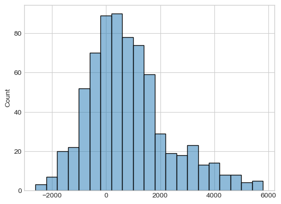
Predict out of bag estimates of the CATE, and create a histogram of these. Do you observe heterogeneity?
Hints:
The documentation for the CausalForest can be found here
Out of bag is sometimes shortened oob
You can create a histogram using sns.histplot
# Your answer here
### BEGIN SOLUTIONtau_cf = cf.oob_predict(X)sns.histplot(tau_cf, legend=False)plt.show()### END SOLUTION
Exercise 1.4
Estimate a CausalForestDML using the econml package. Make sure that you 1) use the splitting criterion as in the generalized random forest, 2) interpret the treatment as a discrete treatment and 3) estimate a thousand trees, but otherwise use default parameters.
Hints:
The documentation for the CausalForestDML can be found here
# Your code here
### BEGIN SOLUTIONfrom econml.dml import CausalForestDMLcf_dml = CausalForestDML( discrete_treatment=True, n_estimators=1000, criterion='het' )cf_dml.fit(Y=y, T=T, X=X)### END SOLUTION
<econml.dml.causal_forest.CausalForestDML at 0x1ff165a1c30>
Exercise 1.5
Report the doubly robust average treatment effect
Hints:
The documentation for the CausalForestDML can be found here
A function which summarizes the model findings is available
# Your code here
### BEGIN SOLUTIONcf_dml.summary()### END SOLUTION
Population summary results are available only if `cache_values=True` at fit time!
Doubly Robust ATE on Training Data Results
point_estimate
stderr
zstat
pvalue
ci_lower
ci_upper
ATE
805.679
487.542
1.653
0.098
-149.886
1761.244
Doubly Robust ATT(T=0) on Training Data Results
point_estimate
stderr
zstat
pvalue
ci_lower
ci_upper
ATT
808.062
473.896
1.705
0.088
-120.757
1736.881
Doubly Robust ATT(T=1) on Training Data Results
point_estimate
stderr
zstat
pvalue
ci_lower
ci_upper
ATT
802.328
965.46
0.831
0.406
-1089.938
2694.594
Exercise 1.6
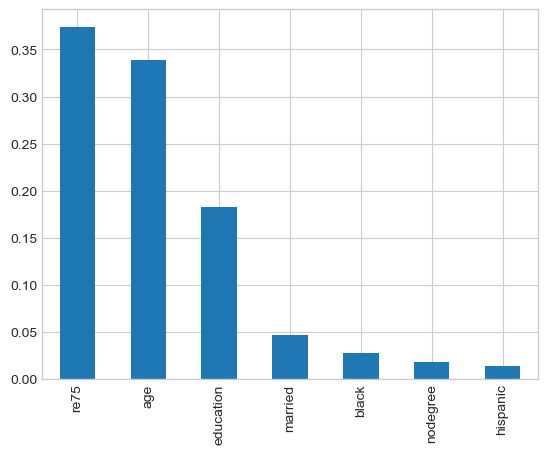
Examine what variables drive the heterogeneity using the split based feature importance method.
Hints:
The documentation for the CausalForestDML can be found here
The feature importances and feature names are available through a method
# Your code here
### BEGIN SOLUTION# Variable name and importance, printed and unsorted for name, importance inzip (cf_dml.cate_feature_names(), cf_dml.feature_importances()):print(f"{name: <10}{importance:.2}")# Sorted and plottedimportances = pd.Series(cf_dml.feature_importances(),index = X.columns).sort_values(ascending=False)importances.plot.bar()plt.show()### END SOLUTION
age        0.34
education  0.18
black      0.027
hispanic   0.013
married    0.046
nodegree   0.018
re75       0.37
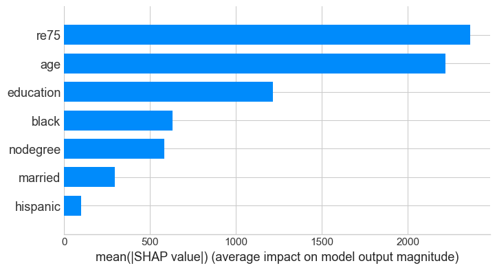
### BEGIN SOLUTIONimport shapunnested_shap_values = shap_values['re78']['treat_1']shap.summary_plot(unnested_shap_values, plot_type="bar")### END SOLUTION
Exercise 1.9
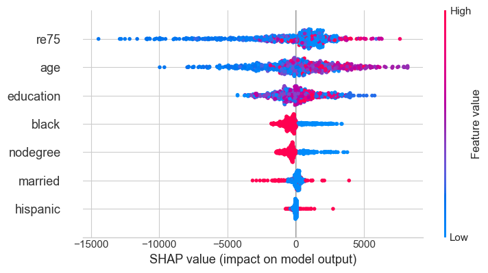
Create a summary plot of the feature importance using SHAP values. In what way does the top variable moderate the CATE?
The feature value colourbar might disappear, in which the following to lines of code might help:
plt.gcf().axes[-1].set_aspect(100)
plt.gcf().axes[-1].set_box_aspect(100)
# Your code here
### BEGIN SOLUTIONshap.summary_plot(unnested_shap_values, show=False)plt.gcf().axes[-1].set_aspect(100)plt.gcf().axes[-1].set_box_aspect(100)### END SOLUTION
Exercise 1.10
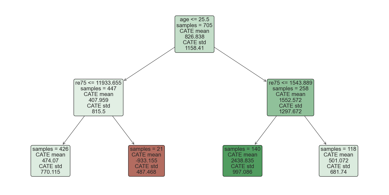
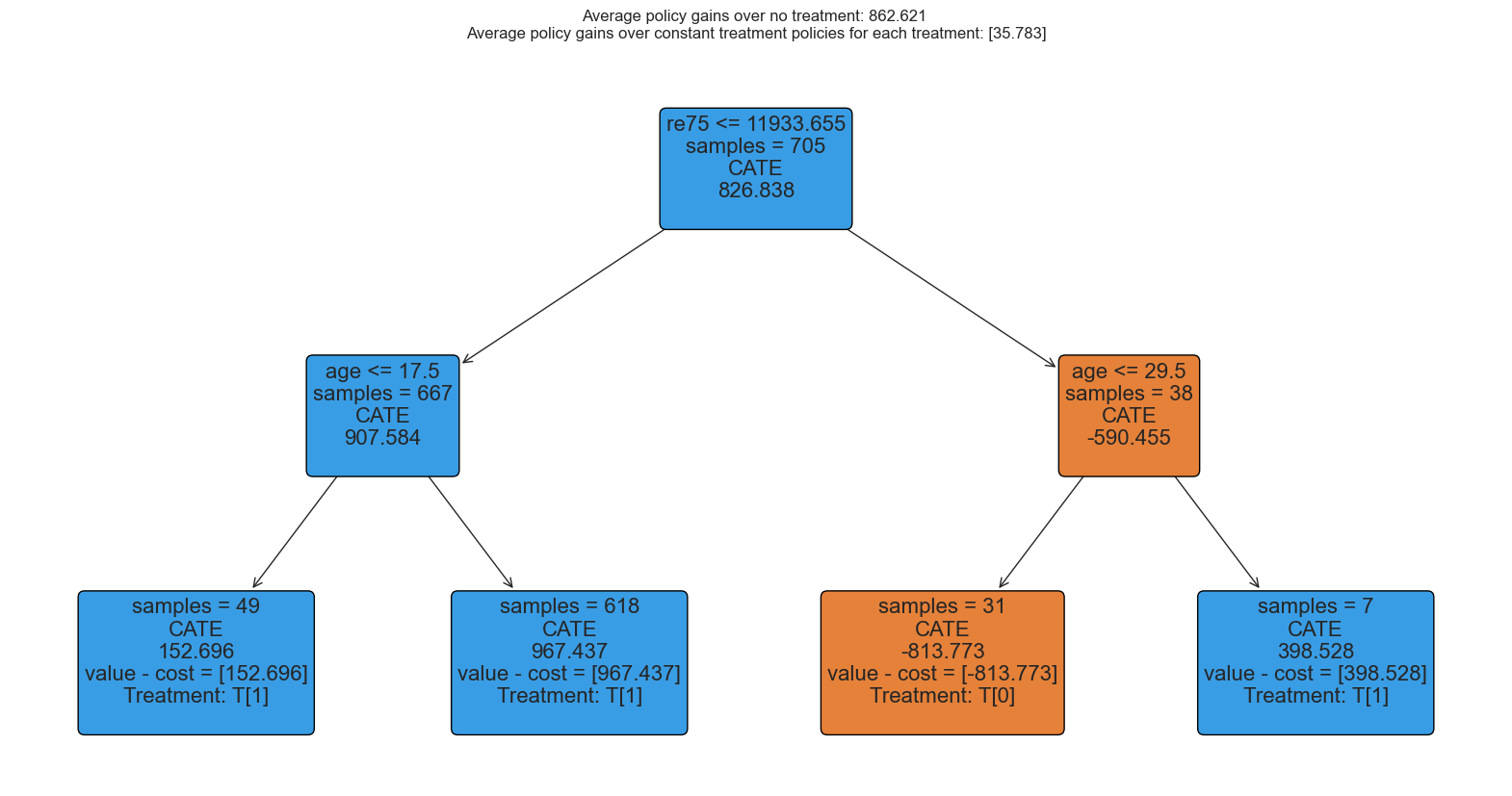
Create a shallow decision tree of depth 2 to explain the CATE as a function of the inputs using SingleTreeCateInterpreter. Does the tree split on the variables you expected it to?
### BEGIN SOLUTIONfrom econml.cate_interpreter import SingleTreePolicyInterpretertreePolicy = SingleTreePolicyInterpreter(max_depth=2)treePolicy.interpret(cf_dml, X)fig, ax = plt.subplots(1, figsize=(20,10))treePolicy.plot(ax=ax, fontsize=16, feature_names=X.columns)### END SOLUTION
R
In the second part of the exercise, we will be utilizing Python and grf. I will supply R code in code that has been commented out (# for code, ## for comments), and they will not be able to run in Python if you comment them in again. One can run R code in Python using rpy2, but I generally recommend using R and not rpy2 due to the complexity of problem solving if rpy2 fails.
The many different functions available in grf can be seen in their reference and they have a lot of great tutorials, accessible at the top of their page.
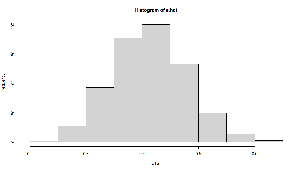
### BEGIN SOLUTION## Treatment propensities#e.hat = cf$W.hat## Plot#hist(e.hat)## Bounded away from 1 and 0, looks good### END SOLUTION
Exercise 2.3
Estimate the doubly robust average treatment effect. Do we find the same as previously?
Hints:
Can you find a function for average treatment effect estimation in the reference?
### BEGIN SOLUTION#average_treatment_effect(cf)## Output## estimate std.err ## 782.0347 508.0461 # Approximately the same as before -- good!### END SOLUTION
Examine what variables drive the heterogeneity using the split based feature importance method.
Hints:
A function to calculate the variable importance can be found in the grf reference
### BEGIN SOLUTION## Calculate variable importance#varimp = variable_importance(cf)## Print results#print(varimp)## [,1]##[1,] 0.29462337##[2,] 0.15099209##[3,] 0.03964410##[4,] 0.01855247##[5,] 0.07758364##[6,] 0.02579878##[7,] 0.39280555## Same results as before, age and re75### END SOLUTION
Exercise 2.9
Examine how the variables affect heterogeneity using the best linear projection.
Hints:
A function to estimate the best linear projection can be found in the grf reference
### BEGIN SOLUTION## Rank vars and get best linear projection#ranked.vars = order(varimp, decreasing = TRUE)#best_lin_proj = best_linear_projection(cf, X[ranked.vars])## Print results#print(best_lin_proj)## Results## Best linear projection of the conditional average treatment effect.##Confidence intervals are cluster- and heteroskedasticity-robust (HC3):#### Estimate Std. Error t value Pr(>|t|) ##(Intercept) -5117.83175 5808.15316 -0.8811 0.378542 ##re75 -0.32801 0.10494 -3.1257 0.001847 **##age 40.38223 80.12389 0.5040 0.614422 ##education 481.73107 383.02820 1.2577 0.208925 ##married 2617.70317 1420.71210 1.8425 0.065822 . ##black 491.84656 1608.76159 0.3057 0.759902 ##nodegree 383.19631 1667.00113 0.2299 0.818259 ##hispanic -818.57994 2099.72022 -0.3899 0.696765 ##---##Signif. codes: 0 ‘***’ 0.001 ‘**’ 0.01 ‘*’ 0.05 ‘.’ 0.1 ‘ ’ 1### END SOLUTION